What would it take to recreate dplyr in python?
February 11, 2020 by Michael Chow
Recently, I left my job as a data scientist at DataCamp to focus full time on two areas:
- co-directing the non-profit Code for Philly
- bringing the magic of dplyr to python
In order to do the second part, I’ve worked over the past year on a data analysis library called siuba. As part of this work, I’ve found myself often discussing siuba’s hardest job: making grouped operations a delight.
In this post I’ll provide a high-level overview of three key challenges for porting dplyr to python. Because the pandas library is the most popular python implementation of both a DataFrame AND performing split-apply-combine on it, I’ll focus mostly on the challenges of building dplyr on top of pandas. Note that all of these challenges arise during the process of split-apply-combine.
Here are the three challenges:
- The index tax - operations that don’t use an index pay to make index copies per group.
- The type conversion tax - Series run slow type checks multiple times per group.
- Grouped operations are not composable - DataFrame and DataFrameGroupBy methods are focused around performing a single action, like calculating a mean. They become verbose when you need to combine actions, like subtracting the mean of a column from itself.
The reason these challenges are important can be illustrated in the dplyr code below.
library(dplyr)
my_arbitrary_func <- function(x) x + 1

# group data by cyl

mtcars %>%
  select(cyl, hp) %>%
  group_by(cyl) %>%
  mutate(
    dumb_result = my_arbitrary_func(hp),     # custom function
    demeaned = hp - mean(hp)                 # complex expression
  )
# A tibble: 32 x 4
# Groups:   cyl [3]
    cyl    hp dumb_result demeaned
  <dbl> <dbl>       <dbl>    <dbl>
1     6   110         111    -12.3
2     6   110         111    -12.3
3     4    93          94     10.4
4     6   110         111    -12.3
5     8   175         176    -34.2
# … with 27 more rows
dplyr absolutely nails two features for grouped operations, even if the data has many groups:
- Allowing people to use custom functions. Eg. fitting a model
- Allowing people to use complex expressions. Eg. subtracting a mean
However, similar expressions in grouped pandas either run very slowly (e.g. 30 seconds for only 50k groups), or require cumbersome syntax. In the following sections, I’ll break down how the index and type conversion taxes make custom functions slow, examine complex expressions in pandas, and finally highlight experimental work with siuba to bridge the gap.
Before starting it’s worth noting that I feel tremendous appreciation for the pandas library, the many challenging problems it tackles, and the time people contribute to it.
Setting up example data #
For this article, I’ll use example data for students receiving scores on a number of courses.
import pandas as pd
from numpy import random
import numpy as np

N_students = 50000
N_courses = 10
user_courses = pd.DataFrame({
    "student_id": np.repeat(range(N_students), N_courses),    # e.g. 1,1,1, ...
    "course_id":  np.tile(range(N_courses), N_students),      # e.g. 1,2,3, ...
    "score": random.randint(0, 100, N_courses*N_students)
})

g_students = user_courses.groupby("student_id")
This data contains 50,000 students who took 10 courses each. Each student received a score between 0 and 100 for each course.
Barriers to customization: the index and type conversion taxes #
Consider a trivial operation: a function that adds 1 to each students score. This doesn’t even require split-apply-combine, but if we did use this approach, we could use a pandas groupby along with two choices…
- whether to use the
.applyor.transformmethod. - whether to add 1 to a group’s Series, or its underlying array.
For example, here is the apply method on a Series.
g_students.apply(lambda d: d.score + 1)
student_id
0           0         100
            1          10
            2          33
            3          45
            4          69
                     ...
49999       499995     72
            499996     74
            499997     54
            499998     10
            499999     86
Name: score, Length: 500000, dtype: int64
Here, we’re returning a Series with the score + 1 (right column). Note that the left two columns are a “multi-index” which is cured using .reset_index–a story for another time. Note also that the .apply method is more general than .transform, which can only be used on a single column of data.
Below is a summary of timings on my laptop for each combination of these choices.
| operation | time |
|---|---|
| apply score + 1 | 30s |
| apply score.values + 1 | 3s |
| transform score + 1 | 30s |
| transform score.values + 1 | 20s |
Notice how using apply on an underlying array, rather than a Series, runs in 1/10th of the time as most other methods!
What could be causing this? At a high-level, there are three factors:
- (split): apply is using a fast method for splitting data
- (split and apply): parts involving Series are very slow
- (combine): the fastest method is actually not performing the combine stage!
It’s worth visiting the last point, before diving more into the first two.
Is the fastest method cheating by not combining? (No) #
I don’t think so, because in practice performing the combine step on it is very fast.
# notice that it isn't returning 500k rows, but 50k rows. One per student.
result = g_students.apply(lambda d: d.score.values + 1)
result.head()
student_id
0       [28, 63, 7, 23, 75, 66, 85, 1, 20, 1]
1    [85, 50, 54, 65, 61, 88, 33, 48, 43, 67]
2       [9, 5, 51, 75, 12, 86, 75, 14, 58, 2]
3      [14, 26, 22, 69, 4, 31, 7, 95, 57, 37]
4     [55, 94, 94, 90, 39, 9, 64, 39, 22, 52]
dtype: object
flat_arr = np.concatenate(list(result))
ser_combined = pd.Series(flat_arr)
ser_combined
0         28
1         63
2          7
3         23
4         75
          ..
499995    11
499996     5
499997    35
499998    29
499999    65
Length: 500000, dtype: int64
On my computer, this takes only about 25 milliseconds–an order of magnitude (or two!) beneath the timings above. As will be discussed more below, combining when done once is not the issue.
Breaking down the index and type taxes for split and apply steps #
While a deep dive into the internals of these methods is a post for another time, I do want to provide a high-level view of what’s going on. A helpful tool in this case is snakeviz, which gives a visual report from profiling code.
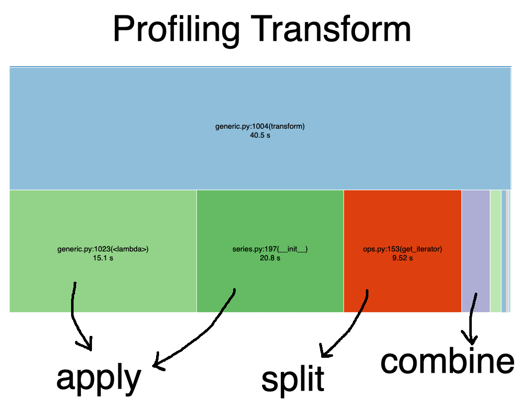
In the graph below, I use the library snakeviz to time g_student.xp.transform(lambda xp: xp + 1).

Note that most of the time is spent on the apply step. Specifically there are two big blocks.
The first is the operation (xp + 1), and the second is pandas remaking a new Series from the result of that operation.
⚠️: the seconds reported in the graphs may not add up, but block sizes should be relatively representative. See this issue.)
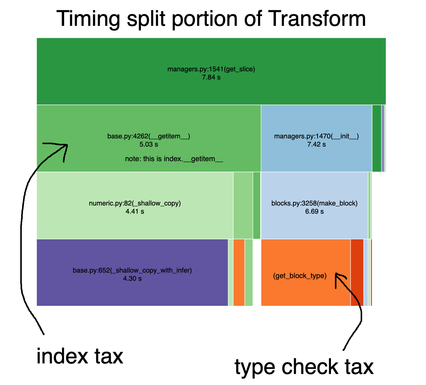
Incredibly, if you look more closely at the time spent splitting, most of the time is spent paying the index and type conversion taxes.

More specifically:
- the index tax: making a shallow copy of every index
- the type conversion tax: inferring the type of the data for each subgroup
In essence, because these taxes are paid once per group in your data (e.g. 50,000, one for each student), they become very hefty.
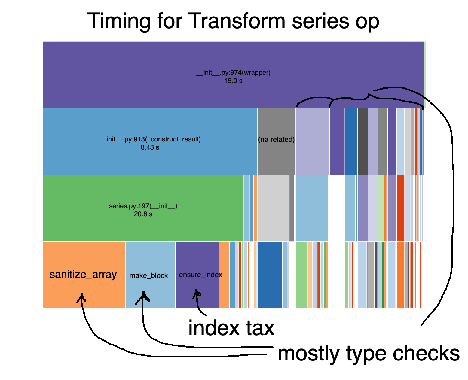
Digging further into the Series operation piece of the apply, xp + 1, we see essentially the same two taxes accumulating for each student group.

The key here is that every time pandas does xp + 1 inside a grouped transform, it is performing it the same as if the data weren’t grouped.
import pandas as pd

ser = pd.Series([1,2,3])
result = ser + 1
Here, it makes sense that pandas might want to do some cumbersome checks–but it makes the custom groupby nearly unusable. This leads us to a critical question: how does pandas implement fast groupby operations?
Grouped operations are not composable #
The key to understanding fast pandas groupby methods, is to realize that they win by not playing the game.
This happens in two ways:
- Running type checks only once, and ignoring index when appropriate (which is often).
- Operate on the underlying array values, or avoid creating a Series for each operation.
This is extremely convenient, but we run into problems when we need to combine these fast methods. They cannot be easily combined.
For instance, consider how simple demeaning a column is in dplyr.
library(dplyr)

mutate(g_students, demeaned = score - mean(score))
# A tibble: 500,000 x 4
# Groups:   student_id [50,000]
  student_id course_id score demeaned
       <dbl>     <dbl> <dbl>    <dbl>
1          0         0    27    -8.90
2          0         1    62    26.1
3          0         2     6   -29.9
4          0         3    22   -13.9
5          0         4    74    38.1
# … with 5e+05 more rows
In pandas, doing the same operation like this looks like…
demeaned = user_courses.score - g_students.score.transform('mean')
user_courses['demeaned'] = demeaned
Two things stick out in the pandas version:
- two objects: we need to refer to both the grouped AND the ungrouped data
- result length dependent operations: to calculate a mean in this case we have to pass the string “mean” to transform. This tells pandas that the result should be the same length as the original data.
In dplyr users don’t need to worry about either of things. dplyr allows users to decouple the specification of operations, result length, and grouping.
Bridging the gap to dplyr with siuba #
In order to decouple operations, result length, and grouping, siuba does two things:
- wraps Series(GroupBy) methods in a way that makes them composable
- uses its port of dplyr verbs, like
mutateto handle result length
from siuba.experimental.pd_groups import fast_mutate
from siuba import _, ungroup

# note: need to ungroup since grouped DataFrames don't have nice repr
fast_mutate(g_students, result = _.score + 1) >> ungroup()
        student_id  course_id  score  demeaned  result
0                0          0     27      -8.9      28
1                0          1     62      26.1      63
...            ...        ...    ...       ...     ...
499998       49999          8     28     -15.9      29
499999       49999          9     64      20.1      65

[500000 rows x 5 columns]
Because it’s a light wrapper around the SeriesGroupBy methods, it runs at roughly the same speed. I’ll write in detail about how it allows users to define their own functions in a future post, but if you’re interested you can read more here in siuba’s docs, or in siuba’s groupby architecture decision doc.
Summary #
The biggest obstacle to implementing a dplyr-like experience in python is figuring how to add flexibility to grouped pandas operations. This is because custom grouped operations exert a high index tax, and type checking tax. Moreover, grouped operations in pandas are not straightforward to combine.
This article has taken a critical look at pandas, but I can’t emphasize enough how useful the library is overall, and appreciate how much time its contributors have spent working out hard problems.
I showed in the article how siuba resolves some of these issues with group by. However, this strategy largely involves wrapping pandas groupoed Series methods. This is because, unlike in R, each splitting and applying a custom operation to a DataFrame or Series is very costly timewise.
In follow-up articles, I will dive more deeply into strategies for more naturally allowing custom operations, by alleviating the index, and type checking tax, so that DataFrames can be quickly split, applied, and combined.
If you have questions about siuba, or grouped operations–feel free reach me on twitter @chowthedog.