Using R and the A* Algorithm: Animated Pathfinding with gganimate

This post is the second part of a series on using the A* algorithm in R.

While my previous post introduced the machow/astar-r library, and how it works, in this one I’ll focus on visualizing it finding a solution with gganimate. Below is an outline of what I’ll cover.

• manually define a maze and plot it with ggplot
• use an example class from the astar library to navigate it
• add a bonus picture of a gnome to the maze
• use a single line of gganimate to animate the A* search

Drawing the maze

First, we’ll load in the necessary libraries, and create a simple maze to navigate.

# Create maze
# remotes::install_github("machow/astar-r")
library(astar)
library(gganimate)
library(dplyr)

M <- matrix(ncol = 8, byrow = TRUE, c(
  0,0,0,0,0,0,1,0,
  0,0,1,1,0,1,1,0,
  1,0,0,0,0,0,1,0,
  0,0,1,1,1,1,1,0,
  1,0,1,0,0,0,0,0,
  0,0,0,0,1,1,0,0
  ))

Note that this task is pretty straightforward. The one important piece that makes it easy to read is setting byrow = TRUE. Otherwise, it will appear rotated 90 degrees.

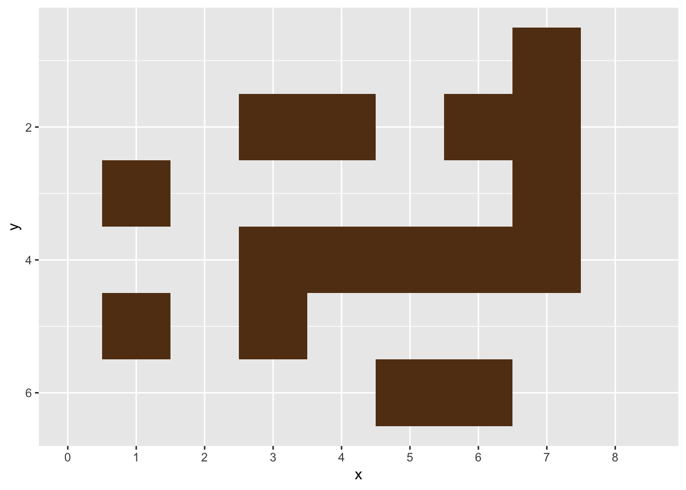
Below, I make a quick plot of the maze, by creating a data.frame where each row is the coordinate of a piece of wall.

walls <-
  which(M == 1, arr.ind = TRUE) %>%
  as.data.frame() %>%
  transmute(y = row, x = col)

walls %>%
  ggplot(aes(x,y)) +
  geom_tile(width = 1, height = 1, fill = "#623B17") +
  scale_y_reverse() +
  scale_x_continuous(breaks = seq(0, 8, 1), limits = c(0, 8.5), minor_breaks = NULL)

Note that the plot uses scale_y_reverse, to take care of the fact that a matrix uses a y index that counts down (e.g. walls[1,] is the top row), but ggplot’s y index counts up.

Navigating through and saving our path

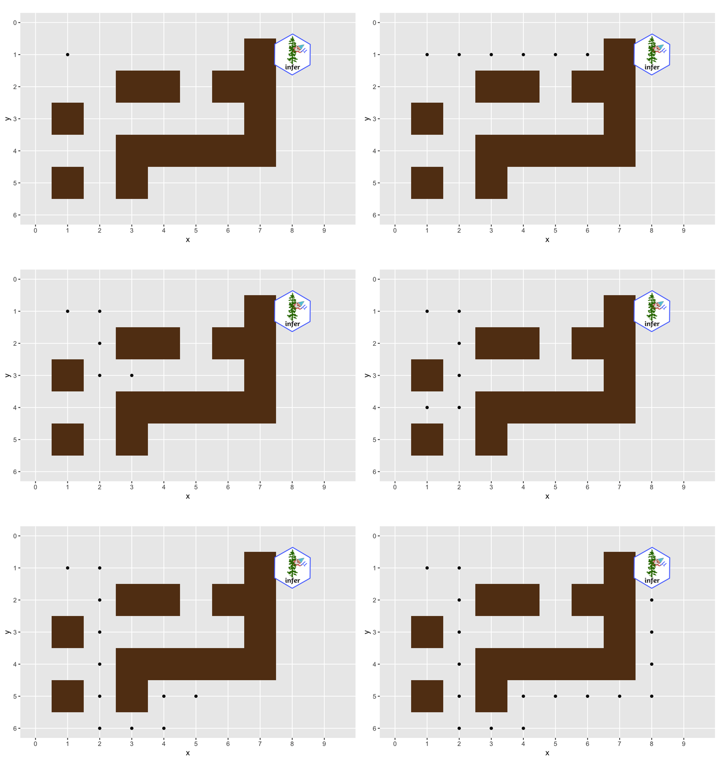
Once the maze is defined, we can use the MazeGazer R6 class to run through it. This class keeps a history of all the spots that the A* algorithm searched from, so we can visualize them later.

# Run maze

mg <- MazeGazer$new(M)
goal_path <- mg$run(c(1,1), c(1,8))

history <- mg$history %>% bind_rows()

head(history)

##   round y x
## 1     1 1 1
## 2     2 1 1
## 3     2 1 2
## 4     3 1 1
## 5     3 1 2
## 6     3 1 3

Note that the astar library has a base class called AStar, that you can use as a template (or subclass) when writing your own tools.

Loading up the infer gnome

Probably the most critical step of the process is loading in the infer gnome hex sticker. Without this sticker, there would be no incentive to get to the end of the maze.

library(png)
library(grid)

# download to computer
gnome <- "https://github.com/tidymodels/infer/raw/master/figs/infer_gnome.png"
download.file(gnome, "./gnome.png")

# load that gnome up!
img <- readPNG("./gnome.png")
g <- rasterGrob(img, interpolate=TRUE)

With gnome in hand, we’re ready to chart our course through the maze.

Making the run!

Below is the code to animate the trip through the maze. Notice that it only needs a single line of gganimate!

ggplot(history, aes(x, y)) +
  # ggplot maze part
  geom_tile(width = 1, height = 1, fill = "#623B17", data = walls) +
  geom_point(aes(group = round)) +
  scale_y_reverse(breaks = seq(6, 0, -1), limits = c(6, 0), minor_breaks = NULL) +
  scale_x_continuous(breaks = seq(0, 100, 1), limits = c(0, 9.5), minor_breaks = NULL) +
  coord_fixed() +
  # ggplot gnome part
  annotation_custom(g, xmin = 7.30, xmax = 8.70, ymin = -.3, ymax = -1.70) +
  # gganimate
  transition_time(round)

Summary

Overall, I was amazed that gganimate is so easy to get into, and did its job in a single line of code! To be sure, it took more lines of code to load the gnome hex sticker than to use gganimate. I’d be curious to know how large the maze (and the history log) can get before making the plot takes too long. I’m also curious if there’s a way with gganimate to only specify the dots we want to add or take away after each round, rather than logging the full path.

If you use the astar package solve any interesting problems, or encounter any bugs, let me know on github! If you have strong opinions on gnomes feel free to share them with me on twitter (@chowthedog).